Matlab
Table of Contents
Matlab 相关的笔记。
<!–more–>
Octave & Matlab
Base
language
注释
% 逐行注释

%%
这里面的内容都被注释
%%

%{这里面的内容都被注释}%
For
  %实例2: 输出1,0.9,。。。。0;这10个数。
  for a = 1.0: -0.1: 0.0
    % 打印变量
    disp(a)
  end
use package
install package
pkg install -forge msh
import and use package
clc
close all
clear all
try
  pkg load matgeom;
catch
  error('Could not load Octave Forge package: matgeom');
end

t = linspace(0, 2*pi, 200);
figure; hold on;
plot(t, sin(t));
drawArrow([2 -1 pi 0], .1, .05, .5);

disp("Hello World");
Use Case
求矩阵逆矩阵
A=[1 2 3;2 2 1;3 4 3];
inv(A);
画对数函数
\(y = log_2x\)
% 绘制以 2 为底的对数函数
x = 0:100;
y = log2(x)
plot(y)
同时画多个函数
% 绘制以 2 为底的对数函数
x = 0:100;
y1 = log2(x);
y2 = x;
plot(x,y1,x,y2);
球面坐标系作图
  %% 清除其他窗口
  clc; clear all; close all;

  theta = linspace(0, pi);
  phi=linspace(0,2*pi);
  [tt,pp]=meshgrid(theta,phi);
  r=max(0,5*cos(theta)-4)+max(0,-4*sin(theta-pi)*cos(pi-2.5)-3);
  [x,y,z]=sph2cart(pp,pi/2-tt,r);

  %% 绘制mesh
  %mesh(x,y,z);
  %% 绘制表面
  surf(x,y,z)
  %% 显示grid
  grid on;
FFT 分析
实现
%%
%% test.m
%%
clear all
clc

fo = 4; %frequency of the sine wave
Fs = 100; %sampling rate
Ts = 1/Fs; %sampling time interval
t = 0:Ts:1-Ts; %sampling period
n = length(t); %number of samples
y = 2*sin(2*pi*fo*t); %the sine curve

subplot(3,1,1);
plot(t,y)
xlabel('time (seconds)')
ylabel('y(t)')
title('Sample Sine Wave')
grid

subplot(3,1,2);
YfreqDomain = fft(y); %take the fft of our sin wave, y(t)

stem(abs(YfreqDomain)); %use abs command to get the magnitude
%similary, we would use angle command to get the phase plot!
%we'll discuss phase in another post though!

xlabel('Sample Number')
ylabel('Amplitude')
title('Using the Matlab fft command')
grid
axis([0,100,0,120])

subplot(3, 1, 3);
[YfreqDomain, freqRange] = centeredFFT(y, Fs);
stem(freqRange, abs(YfreqDomain));
xlabel('Hz')
ylabel("Amplitude")
grid
axis([-6,6,0,1.5])

%%
%% centeredFFT.m
%%
function [X,freq]=centeredFFT(x,Fs)
    %this is a custom function that helps in plotting the two-sided spectrum
    %x is the signal that is to be transformed
    %Fs is the sampling rate

    N=length(x);

    %this part of the code generates that frequency axis
    if mod(N,2)==0
    k=-N/2:N/2-1; % N even
    else
    k=-(N-1)/2:(N-1)/2; % N odd
    end
    T=N/Fs;
    freq=k/T; %the frequency axis

    %takes the fft of the signal, and adjusts the amplitude accordingly
    X=fft(x)/N; % normalize the data
    X=fftshift(X); %shifts the fft data so that it is centered
end
函数说明
stem
stem
stem(Y) 将数据序列Y从x轴到数据值按照茎状形式画出,以圆圈终止。如果Y是一个矩阵,则将其每一列按照分隔方式画出。
stem(X,Y)在X的指定点处画出数据序列Y.
stem(...,'filled') 以实心的方式画出茎秆。
stem(...,'LINESPEC') 按指定的线型画出茎秆及其标记
参考资料
- Matlab 进行 FFT 分析 https://www.jianshu.com/p/0c05d99f7e8a
- 如何使用 matlab 进行频域分析 https://zhuanlan.zhihu.com/p/42893470
Mathematica
显示坐标轴
Plot3D[0.5 (1/(E^((1 - x^2)/(x^2 y^2)) x^4 y^2))^0.1, {x, 0, 1}, {y, 0, 1}, AxesLabel -> {x 轴, y 轴, z 轴}]
WolframAlpha
求积分
integrate sin x dx from x=0 to pi
解方程组
0.3290 * w = 1, 0.6400 * r + 0.3*g + 0.15*b = 0.3127*w, 0.3300 * r + 0.6*g + 0.06*b = 0.3290*w, 0.0300 * r + 0.1*g + 0.79*b = 0.3583*w
矩阵运算
// Von Kries
{{0.4002, 0.7076, -0.0808},{-0.2263,1.1653,0.0457},{0,0,0.9182}} * {0.950455, 0.999999, 1.08906}
==> (0.999976, 0.999982, 0.999975)

// CIECAM02
{{0.7328f, 0.4296f, -0.1624f},{-0.7036f, 1.6975f,  0.0061f},{ 0.0030f, 0.0136f,  0.9834f}} * {0.950455, 0.999999, 1.08906}
==> (0.94923 f, 1.0354 f, 1.08743 f)
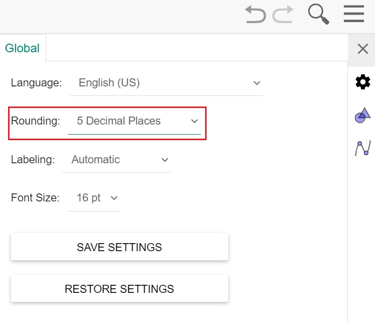
GeoGebra
常用功能
设置
设置小数点精度
使用
// 设置函数定义域、值域
y=x^(2) (0<x<1)
y=x (0<y<1)

// 分段函数
y21(x) = if(x<0.3,0,x>0.9,0,(1-j)/x)

// 求交点
rts11 = Intersect(y21, x = l)

// 获取点的 x 分量 y 分量
x(P)
y(P)

// 输入无穷大
\infinite
极坐标图像
// 格式: Curve((ρ(θ);θ), θ, α, β)

// 实例: Curve((a * 1 + cos²(θ); θ), θ, 0, 2π)
List
// 定义EValueList
EValueList = Sequence(-5, 5)

// 取List中第i个元素   // Element(EValueList, i)
// 取 List 的元素数量      // Length(EValueList)
precision = Sequence(Segment((i, 0), (i, 2^(Element(EValueList, i) - 23) * 200)), i, 1, Length(EValueList))
Sequence
生成一系列点
samples = Sequence((k, 0), k, 0.1, 1.9, 0.2)
Vector Matrix
pos = (1,1,1)

matScale = {{rFactor, 0, 0}, {0, gFactor, 0}, {0, 0, bFactor}}

scaledPos = matScale * pos
ERROR
垂线不正确
这是因为 x 和 y 轴的缩放比例不为 1:1 导致的。